np.linspace(): Create Evenly or Non-Evenly Spaced Arrays

Using np.linspace()

np.linspace() has two required parameters, start and stop, which you can use to set the beginning and end of the range:

>>> import numpy as np
>>> np.linspace(1, 10)
array([ 1.        ,  1.18367347,  1.36734694,  1.55102041,  1.73469388,
        1.91836735,  2.10204082,  2.28571429,  2.46938776,  2.65306122,
        2.83673469,  3.02040816,  3.20408163,  3.3877551 ,  3.57142857,
        3.75510204,  3.93877551,  4.12244898,  4.30612245,  4.48979592,
        4.67346939,  4.85714286,  5.04081633,  5.2244898 ,  5.40816327,
        5.59183673,  5.7755102 ,  5.95918367,  6.14285714,  6.32653061,
        6.51020408,  6.69387755,  6.87755102,  7.06122449,  7.24489796,
        7.42857143,  7.6122449 ,  7.79591837,  7.97959184,  8.16326531,
        8.34693878,  8.53061224,  8.71428571,  8.89795918,  9.08163265,
        9.26530612,  9.44897959,  9.63265306,  9.81632653, 10.        ])

This code returns an ndarray with equally spaced intervals between the start and stop values. This is a vector space, also called a linear space, which is where the name linspace comes from.

Note that the value 10 is included in the output array. The function returns a closed range, one that includes the endpoint, by default. This is contrary to what you might expect from Python, in which the end of a range usually isn’t included. This break with convention isn’t an oversight. You’ll see later on that this is usually what you want when using this function.

The array in the example above is of length 50, which is the default number. In most cases, you’ll want to set your own number of values in the array. You can do so with the optional parameter num:

>>> np.linspace(1, 10, num=10)
array([ 1.,  2.,  3.,  4.,  5.,  6.,  7.,  8.,  9., 10.])

The output array in this instance contains 10 equally spaced values between 1 and 10, which is just the numbers from 1 to 10. Here’s another example:

>>> np.linspace(-10, 10, 25)
array([-10.        ,  -9.16666667,  -8.33333333,  -7.5       ,
        -6.66666667,  -5.83333333,  -5.        ,  -4.16666667,
        -3.33333333,  -2.5       ,  -1.66666667,  -0.83333333,
         0.        ,   0.83333333,   1.66666667,   2.5       ,
         3.33333333,   4.16666667,   5.        ,   5.83333333,
         6.66666667,   7.5       ,   8.33333333,   9.16666667,
        10.        ])

In the example above, you create a linear space with 25 values between -10 and 10. You use the num parameter as a positional argument, without explicitly mentioning its name in the function call. This is the form you’re likely to use most often.

Using range() and List Comprehensions

Let’s take a step back and look at what other tools you could use to create an evenly spaced range of numbers. The most straightforward option that Python offers is the built-in range(). The function call range(10) returns an object that produces the sequence from 0 to 9, which is an evenly spaced range of numbers.

For many numerical applications, the fact that range() is limited to integers is too restrictive. Of the examples shown above, only np.linspace(1, 10, 10) can be accomplished with range():

>>> list(range(1, 11))
[1, 2, 3, 4, 5, 6, 7, 8, 9, 10]

The values returned by range(), when converted explicitly into a list, are the same as those returned by the NumPy version, except that they’re integers instead of floats.

You can still use range() with list comprehensions to create non-integer ranges:

>>> step = 20 / 24  # Divide the range into 24 intervals
>>> [-10 + step*interval for interval in range(25)]
[-10.0, -9.166666666666666, -8.333333333333334, -7.5,
 -6.666666666666666, -5.833333333333333, -5.0, -4.166666666666666,
 -3.333333333333333, -2.5, -1.666666666666666, -0.8333333333333321,
 0.0, 0.8333333333333339, 1.6666666666666679, 2.5,
 3.333333333333334, 4.166666666666668, 5.0, 5.833333333333334,
 6.666666666666668, 7.5, 8.333333333333336, 9.166666666666668, 10.0]

The values in the list are the same as the values in the array outputted by np.linspace(-10, 10, 25). However, even using a list comprehension is rather clumsy and inelegant compared to using np.linspace(). You first need to work out the interval required and then use that interval within a loop.

In most applications, you’ll still need to convert the list into a NumPy array since element-wise computations are less complicated to perform using NumPy arrays.

Another point you may need to take into account when deciding whether to use NumPy tools or core Python is execution speed. You can expand the section below to see how using a list performs in comparison to using a NumPy array.

 1>>> import timeit
 2>>> import numpy as np
 3>>> numbers_array = np.linspace(-10, 10, 500)
 4>>> step = 20 / 499
 5>>> numbers_list = [-10 + step*interval for interval in range(500)]
 6>>> def test_np():
 7...     return (numbers_array + 2.5) ** 2
 8...
 9>>> def test_list():
10...     return [(number + 2.5) ** 2 for number in numbers_list]
11...
12>>> list(test_np()) == test_list()
13True
14>>> timeit.timeit("test_np()", globals=globals(), number=100000)
150.3116540400000076
16>>> timeit.timeit("test_list()", globals=globals(), number=100000)
175.478577034000011

Using NumPy tools rather than core Python can yield efficiency gains in some instances. In applications that require many computations on large amounts of data, this increase in efficiency can be significant.

Using np.arange()

NumPy has its own version of the built-in range(). It’s called np.arange(), and unlike range(), it’s not restricted to just integers. You can use np.arange() in a similar way to range(), using start, stop, and step as the input parameters:

>>> list(range(2, 30, 2))
[2, 4, 6, 8, 10, 12, 14, 16, 18, 20, 22, 24, 26, 28]

>>> np.arange(2, 30, 2)
array([ 2,  4,  6,  8, 10, 12, 14, 16, 18, 20, 22, 24, 26, 28])

The output values are the same, although range() returns a range object, which can be converted to a list to display all the values, while np.arange() returns an array.

The array returned by np.arange() uses a half-open interval, which excludes the endpoint of the range. This behavior is similar to range() but different from np.linspace(). These differences can be a bit confusing initially, but you’ll get used to them as you start using these functions more often.

You can even use non-integer numbers with np.arange():

>>> np.arange(2.34, 31.97, 2)
array([ 2.34,  4.34,  6.34,  8.34, 10.34, 12.34, 14.34, 16.34, 18.34,
       20.34, 22.34, 24.34, 26.34, 28.34, 30.34])

The output is an array starting from the start value, with the gap between each number being exactly equal to the step size used in the input arguments. The last number is the largest number in this series that is smaller than the number used for the end of the range.

The step argument can also be a floating-point number, although you’ll need to use caution in this case as the output may not always be quite what you intend:

>>> np.arange(1.034, 3.104, 0.34)
array([1.034, 1.374, 1.714, 2.054, 2.394, 2.734, 3.074])

>>> np.arange(1.034, 3.104, 0.345)
array([1.034, 1.379, 1.724, 2.069, 2.414, 2.759, 3.104])

In the first example, everything seems fine. However, you may have noticed that in the second example, when the step is 0.345, the last value in the output is equal to the stop value even though np.arange() uses a half-open interval. The documentation for np.arange() has a warning about this:

When using a non-integer step, such as 0.1, the results will often not be consistent. It is better to use numpy.linspace for these cases. (Source)

Here’s a good rule of thumb for deciding which of the two functions to use:

• Use np.linspace() when the exact values for the start and end points of your range are the important attributes in your application.
• Use np.arange() when the step size between values is more important.

You’ll use np.arange() again in this tutorial. To learn more about it, check out NumPy arange(): How to Use np.arange().

The start, stop, and num Parameters

Although start and stop are the only required parameters, you’ll usually also want to use a third parameter, num. The parameters start and stop are the beginning and end of the range you wish to create, and num is an integer that determines how many elements the output array will have.

Depending on the application you’re developing, you may think of num as the sampling, or resolution, of the array you’re creating. Have a look at a few more examples:

>>> np.linspace(-5, 5, 10)
array([-5.        , -3.88888889, -2.77777778, -1.66666667, -0.55555556,
        0.55555556,  1.66666667,  2.77777778,  3.88888889,  5.        ])

>>> np.linspace(-5, 5, 100)
array([-5.        , -4.8989899 , -4.7979798 , -4.6969697 , -4.5959596 ,
       -4.49494949, -4.39393939, -4.29292929, -4.19191919, -4.09090909,
       -3.98989899, -3.88888889, -3.78787879, -3.68686869, -3.58585859,
       -3.48484848, -3.38383838, -3.28282828, -3.18181818, -3.08080808,
       -2.97979798, -2.87878788, -2.77777778, -2.67676768, -2.57575758,
       -2.47474747, -2.37373737, -2.27272727, -2.17171717, -2.07070707,
       -1.96969697, -1.86868687, -1.76767677, -1.66666667, -1.56565657,
       -1.46464646, -1.36363636, -1.26262626, -1.16161616, -1.06060606,
       -0.95959596, -0.85858586, -0.75757576, -0.65656566, -0.55555556,
       -0.45454545, -0.35353535, -0.25252525, -0.15151515, -0.05050505,
        0.05050505,  0.15151515,  0.25252525,  0.35353535,  0.45454545,
        0.55555556,  0.65656566,  0.75757576,  0.85858586,  0.95959596,
        1.06060606,  1.16161616,  1.26262626,  1.36363636,  1.46464646,
        1.56565657,  1.66666667,  1.76767677,  1.86868687,  1.96969697,
        2.07070707,  2.17171717,  2.27272727,  2.37373737,  2.47474747,
        2.57575758,  2.67676768,  2.77777778,  2.87878788,  2.97979798,
        3.08080808,  3.18181818,  3.28282828,  3.38383838,  3.48484848,
        3.58585859,  3.68686869,  3.78787879,  3.88888889,  3.98989899,
        4.09090909,  4.19191919,  4.29292929,  4.39393939,  4.49494949,
        4.5959596 ,  4.6969697 ,  4.7979798 ,  4.8989899 ,  5.        ])

Both arrays represent the range between -5 and 5 but with different sampling, or resolution. If you prefer, you can use named parameters:

>>> np.linspace(start=-5, stop=5, num=10)
array([-5.        , -3.88888889, -2.77777778, -1.66666667, -0.55555556,
        0.55555556,  1.66666667,  2.77777778,  3.88888889,  5.        ])

The use of named parameters makes the code more readable. In many applications that use np.linspace() extensively, however, you’ll most often see it used without the first three parameters being named.

You can use non-integer numbers to define the range:

>>> np.linspace(-5.2, 7.7, 30)
array([-5.2       , -4.75517241, -4.31034483, -3.86551724, -3.42068966,
       -2.97586207, -2.53103448, -2.0862069 , -1.64137931, -1.19655172,
       -0.75172414, -0.30689655,  0.13793103,  0.58275862,  1.02758621,
        1.47241379,  1.91724138,  2.36206897,  2.80689655,  3.25172414,
        3.69655172,  4.14137931,  4.5862069 ,  5.03103448,  5.47586207,
        5.92068966,  6.36551724,  6.81034483,  7.25517241,  7.7       ])

The array now consists of 30 equally spaced numbers starting and stopping at the exact values used as arguments for the start and stop parameters. You now know how to use the three main input parameters:

1. start
2. stop
3. num

Often, you’ll use this function with only these three input parameters. However, as you’ll see in the next sections, you can modify the output further.

The dtype Parameter for Changing Output Type

The elements of a NumPy array all belong to the same data type. np.linspace() typically returns arrays of floats. You can see this both by inspecting the output or, better still, by looking at the .dtype attribute for the array:

>>> numbers = np.linspace(-10, 10, 20)
>>> numbers
array([-10.        ,  -8.94736842,  -7.89473684,  -6.84210526,
        -5.78947368,  -4.73684211,  -3.68421053,  -2.63157895,
        -1.57894737,  -0.52631579,   0.52631579,   1.57894737,
         2.63157895,   3.68421053,   4.73684211,   5.78947368,
         6.84210526,   7.89473684,   8.94736842,  10.        ])

>>> numbers.dtype
dtype('float64')

The numbers in the array are floats. This is true even in cases such as the following:

>>> numbers = np.linspace(-10, 10, 11)
>>> numbers
array([-10.,  -8.,  -6.,  -4.,  -2.,   0.,   2.,   4.,   6.,   8.,  10.])

>>> numbers.dtype
dtype('float64')

Even though all elements are whole numbers, they’re still displayed with a trailing period to show that they’re floats. You confirm that by looking at the value of numbers.dtype.

You can use the optional dtype input parameter to change the data type of the elements in the output array:

>>> numbers = np.linspace(-10, 10, 11, dtype=int)
>>> numbers
array([-10,  -8,  -6,  -4,  -2,   0,   2,   4,   6,   8,  10])

>>> numbers.dtype
dtype('int64')

Although the argument states dtype=int, NumPy interprets this as an int64, which is a data type within NumPy. You can confirm this by checking the type of one of the elements of numbers:

>>> type(numbers[0])
<class 'numpy.int64'>

This shows that NumPy uses its own version of the basic data types. You can use the NumPy data types directly as an argument for the dtype parameter:

numbers = np.linspace(-10, 10, 11, dtype=np.int64)

This produces the same output result but avoids ambiguity by explicitly stating the NumPy data type.

When choosing a specific data type, you need to use caution to make sure that your linear space is still valid:

>>> np.linspace(-5, 5, 20, dtype=np.int64)
array([-5, -4, -3, -3, -2, -2, -1, -1,  0,  0,  0,  0,  1,  1,  2,  2,  3,
        3,  4,  5])

NumPy forces the values to be of type np.int64 by rounding in the usual manner, but the result is no longer a linear space. It’s unlikely that this is the outcome you want. You can read more on data types in NumPy in the official documentation.

The endpoint and retstep Parameters

By default, np.linspace() uses a closed interval, [start, stop], in which the endpoint is included. This will often be your desired way of using this function. However, if you need to create a linear space with a half-open interval, [start, stop), then you can set the optional Boolean parameter endpoint to False:

>>> np.linspace(-5, 5, 20, endpoint=False)
array([-5. , -4.5, -4. , -3.5, -3. , -2.5, -2. , -1.5, -1. , -0.5,  0. ,
        0.5,  1. ,  1.5,  2. ,  2.5,  3. ,  3.5,  4. ,  4.5])

This option allows you to use the function with the Python convention of not including the endpoint with a range.

The function can also output the size of the interval between samples that it calculates. If you need the value of the step size between elements, then you can set the Boolean parameter retstep to True:

>>> numbers, step = np.linspace(-5, 5, 20, retstep=True)
>>> numbers
array([-5.        , -4.47368421, -3.94736842, -3.42105263, -2.89473684,
       -2.36842105, -1.84210526, -1.31578947, -0.78947368, -0.26315789,
        0.26315789,  0.78947368,  1.31578947,  1.84210526,  2.36842105,
        2.89473684,  3.42105263,  3.94736842,  4.47368421,  5.        ])

>>> step
0.5263157894736842

The return value in this case is a tuple with the array as the first element and a float with the step size as the second.

Nonscalar Values for Higher-Dimensional Arrays

You can also use nonscalar values for start and stop. This returns a higher-dimensional array:

>>> output = np.linspace(start=[2, 5, 9], stop=[100, 130, 160], num=10)
>>> output
array([[  2.        ,   5.        ,   9.        ],
       [ 12.88888889,  18.88888889,  25.77777778],
       [ 23.77777778,  32.77777778,  42.55555556],
       [ 34.66666667,  46.66666667,  59.33333333],
       [ 45.55555556,  60.55555556,  76.11111111],
       [ 56.44444444,  74.44444444,  92.88888889],
       [ 67.33333333,  88.33333333, 109.66666667],
       [ 78.22222222, 102.22222222, 126.44444444],
       [ 89.11111111, 116.11111111, 143.22222222],
       [100.        , 130.        , 160.        ]])

>>> output.shape
(10, 3)

Both start and stop are lists of the same length. The first items from each list, 2 and 100, are the start and stop points for the first vector, which has 10 samples as determined by the num parameter. The same applies for the second elements from each list and the third ones. The output is a two-dimensional NumPy array with ten rows and three columns.

You can explore this array further by inspecting a row and an element from the two-dimensional array:

>>> output[0]
array([2., 5., 9.])

>>> output[0][2]
9.0

The first result represents the first row of the array. The second result shows the element in the third column of the first row.

You can return the transposed version of this array by setting the optional parameter axis to 1:

>>> output = np.linspace(start=[2, 5, 9],
...                      stop=[100, 130, 160],
...                      num=10,
...                      axis=1)
>>> output
array([[  2.        ,  12.88888889,  23.77777778,  34.66666667,
         45.55555556,  56.44444444,  67.33333333,  78.22222222,
         89.11111111, 100.        ],
       [  5.        ,  18.88888889,  32.77777778,  46.66666667,
         60.55555556,  74.44444444,  88.33333333, 102.22222222,
        116.11111111, 130.        ],
       [  9.        ,  25.77777778,  42.55555556,  59.33333333,
         76.11111111,  92.88888889, 109.66666667, 126.44444444,
        143.22222222, 160.        ]])

>>> output.shape
(3, 10)

The output array now has the number of rows and columns swapped relative to the earlier example, in which the axis parameter was not explicitly set and the default value of 0 was used.

Summary of Input Parameters and Return Values

The function declaration serves as a good summary of the options at your disposal:

linspace(start,
         stop,
         num=50,
         endpoint=True,
         retstep=False,
         dtype=None,
         axis=0
         )

You can find the full details in the documentation. The key points to remember about the input parameters are listed below:

The outputs returned from calling the function are listed below:

• An array of type ndarray containing the vector space
• The step size as a float, if retstep is set to True

You can use this section as a reference when you start experimenting with np.linspace() and the different ways you can customize its output.

Example: A Food Production Conveyor Belt

Imagine that a company that produces packaged food items has a conveyor belt system in its food production factory. The position along the conveyor belt is referenced by a number that represents the length of the conveyor path from the starting point. There are 27 temperature sensors that have been installed at equal intervals along a critical stretch of the belt. The first sensor is located at position 17.5 along the belt, and the last one at 46.2.

The temperature sensor array outputs data that can be read as a list in Python. Here’s an example of a readout of temperatures in degrees Celsius:

temperatures = [17.6, 18.9, 18.0, 18.9, 16.7, 14.3, 13.7, 13.8, 13.6, 15.7,
                18.6, 17.5, 18.4, 18.0, 17.2, 16.9, 16.8, 17.0, 15.9, 17.2,
                17.7, 16.9, 17.2, 17.8, 17.5, 16.9, 17.2]

The factory manager needs to see these temperatures plotted against their position on the conveyor belt to ensure temperatures remain within tolerance at each point on this critical stretch of the belt.

You’ll need to import matplotlib to plot the temperatures:

import matplotlib.pyplot as plt

temperatures = [17.6, 18.9, 18.0, 18.9, 16.7, 14.3, 13.7, 13.8, 13.6, 15.7,
                18.6, 17.5, 18.4, 18.0, 17.2, 16.9, 16.8, 17.0, 15.9, 17.2,
                17.7, 16.9, 17.2, 17.8, 17.5, 16.9, 17.2]

plt.plot(temperatures)
plt.title("Temperatures along critical stretch (ºC)")
plt.ylabel("Temperature (ºC)")
plt.xlabel("List index")
plt.show()

You plot the values in the temperatures list and set the title and axis labels. This gives the following plot:

This plot shows the temperatures plotted against the list index of the sensors. This isn’t useful for the factory manager, who wants to know the temperatures with respect to the standard reference positions of the belt.

To create an index for the temperatures that matches the known reference positions, you’ll use three bits of information:

1. There are 27 temperature sensors.
2. The first one is at position 17.5.
3. The last one is at position 46.2.

This is an ideal scenario for using np.linspace():

>>> import numpy as np
>>> position = np.linspace(17.5, 46.2, 27)
>>> position
array([17.5       , 18.60384615, 19.70769231, 20.81153846, 21.91538462,
       23.01923077, 24.12307692, 25.22692308, 26.33076923, 27.43461538,
       28.53846154, 29.64230769, 30.74615385, 31.85      , 32.95384615,
       34.05769231, 35.16153846, 36.26538462, 37.36923077, 38.47307692,
       39.57692308, 40.68076923, 41.78461538, 42.88846154, 43.99230769,
       45.09615385, 46.2       ])

The linear space position shows the exact locations of all the temperature sensors along the conveyor belt. You can now plot the temperatures against the position array:

plt.plot(position, temperatures)
plt.title("Temperatures along critical stretch (ºC)")
plt.ylabel("Temperature (ºC)")
plt.xlabel("Position on conveyor belt")
plt.show()

The difference from the previous example in the code above is that you use the position array as the first argument in plt.plot(). This gives the following plot:

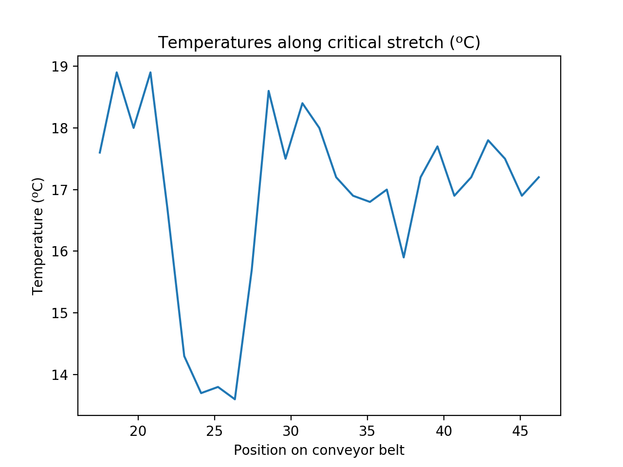
The graph now shows the correct x-axis, which represents the positions at which each temperature was measured. This example shows a typical case for which np.linspace() is the ideal solution.

Mathematical Functions With np.linspace()

In this section, you’ll learn how to represent a mathematical function in Python and plot it. Consider the following function:

This mathematical function is a mapping from the continuous real number line. Even if limits are set, say for -5 ≤ x ≤ 5, there is still an infinite number of values of x. To represent the function above, you’ll first need to create a discrete version of the real number line:

import numpy as np

x_ = np.linspace(-5, 5, 5)

In this tutorial, the symbol x is used to represent the continuous mathematical variable defined over the real number line, and x_ is used to represent the computational, discrete approximation of it. The version with an underscore is also used for the Python variable representing the array.

Since x_ is a NumPy array, you can compute algebraic manipulations similarly to how you would mathematically, and no loops are required:

y_ = 4 * (x_**3) + 2 * (x_**2) + 5 * x_

The new array, y_, is a discrete version of the continuous variable y. The final step is to visualize it:

import matplotlib.pyplot as plt

plt.plot(x_, y_)
plt.show()

This creates a plot of y_ against x_, which is shown below:

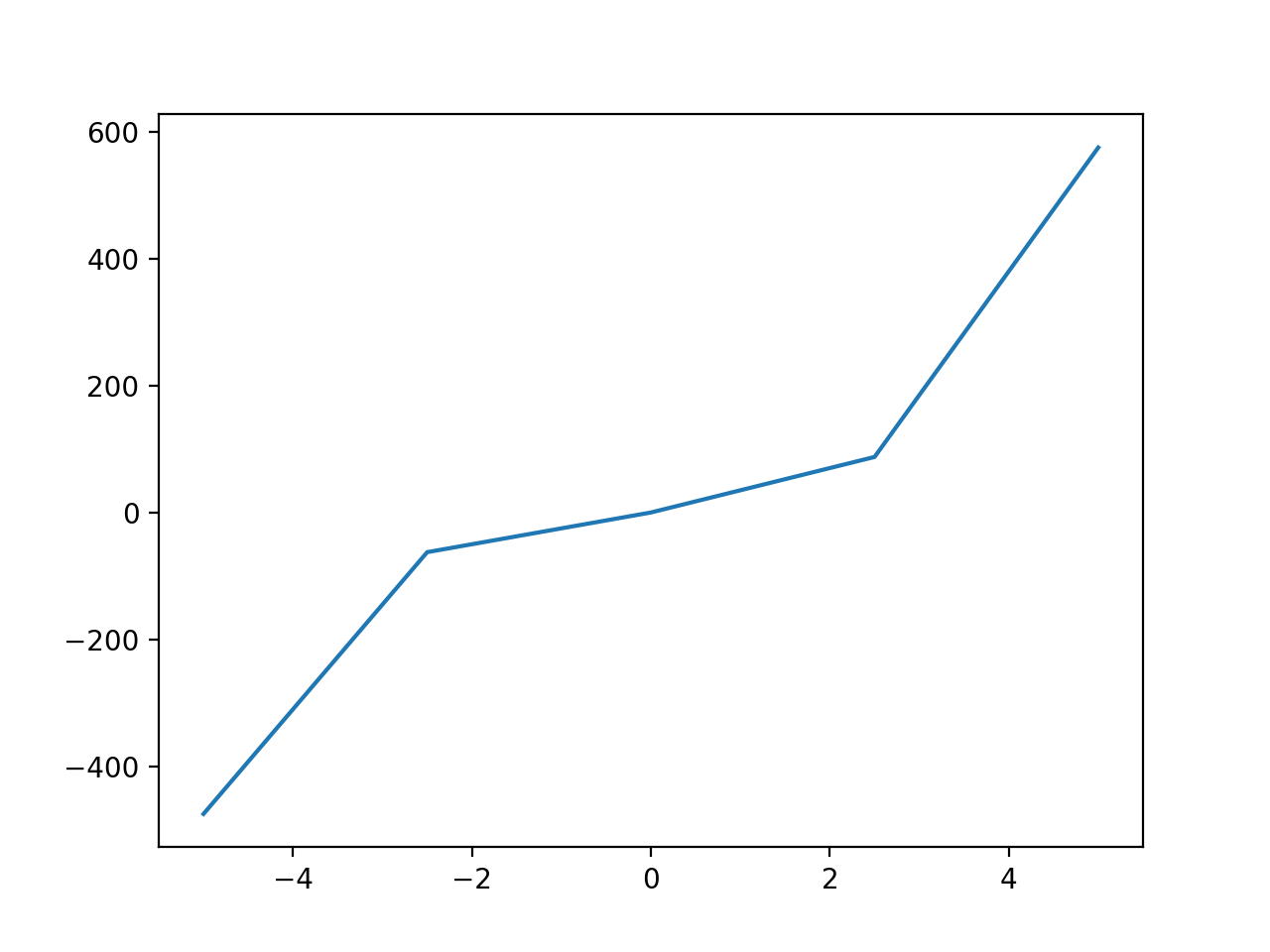
Note that this plot doesn’t seem very smooth. The linear space created has only 5 points. That’s not enough to represent the mathematical function properly. The function is undersampled. Doubling the resolution may work better:

x_ = np.linspace(-5, 5, 10)
y_ = 4 * (x_**3) + 2 * (x_**2) + 5 * x_
plt.plot(x_, y_)
plt.show()

This gives the following plot:

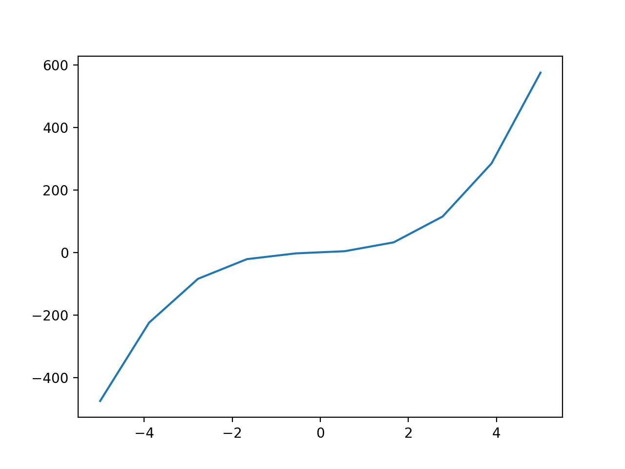
That’s better, and you can be more confident that it’s a fair representation of the function. However, the plot still isn’t as smooth as you might expect to see in a math textbook. With an even higher sampling, the plot becomes smoother:

x_ = np.linspace(-5, 5, 100)
y_ = 4 * (x_**3) + 2 * (x_**2) + 5 * x_
plt.plot(x_, y_)
plt.show()

This gives the following plot:

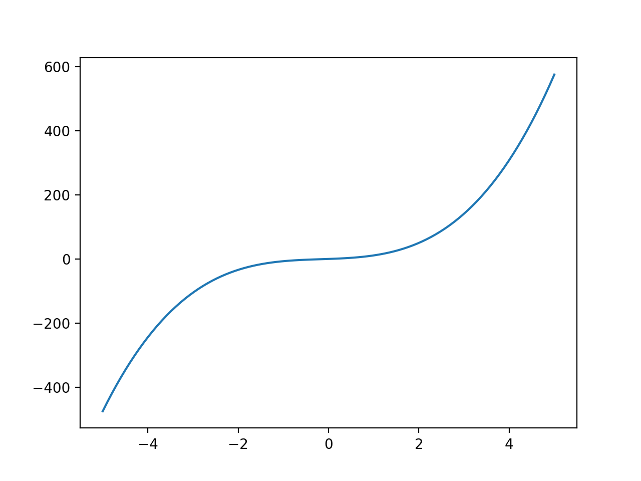
You can choose an even higher sampling, but that will come at a cost. Larger arrays require more memory, and computations will require more time.

Example: Superimposing Traveling Waves

In this section, you’ll create two different waves with distinct properties, then you’ll superimpose them and create an animation to show how they travel.

A wave can be represented mathematically by the following function:

This tutorial isn’t about the physics of waves, so I’ll keep the physics very brief! A wave follows a sinusoidal function that is defined by the following five terms:

• The position (x)
• The time (t)
• The amplitude of the wave (A)
• The wavelength (λ)
• The velocity of the wave (v)

You’ll learn how to deal with two-dimensional functions in the next section, but for this example you’ll take a different approach. You can start by creating a linear space to represent x:

import numpy as np

x_ = np.linspace(-10, 10, 10)

Once the constants are defined, you can create the wave. You can start by defining the constants:

amplitude = 2
wavelength = 5
velocity = 2

time = 0  # You can set time to 0 for now

The function includes time (t), but initially you’ll focus on the variable x. Setting time = 0 for now means that you can still write the full equations in your code even though you’re not using time yet. You can now create the array to represent the wave:

wave = amplitude * np.sin((2*np.pi/wavelength) * (x_ - velocity*time))

The array created is the discrete version of the equation that describes the wave. Now you can plot the wave:

import matplotlib.pyplot as plt

plt.plot(x_, wave)
plt.show()

The plot of the wave is shown below:

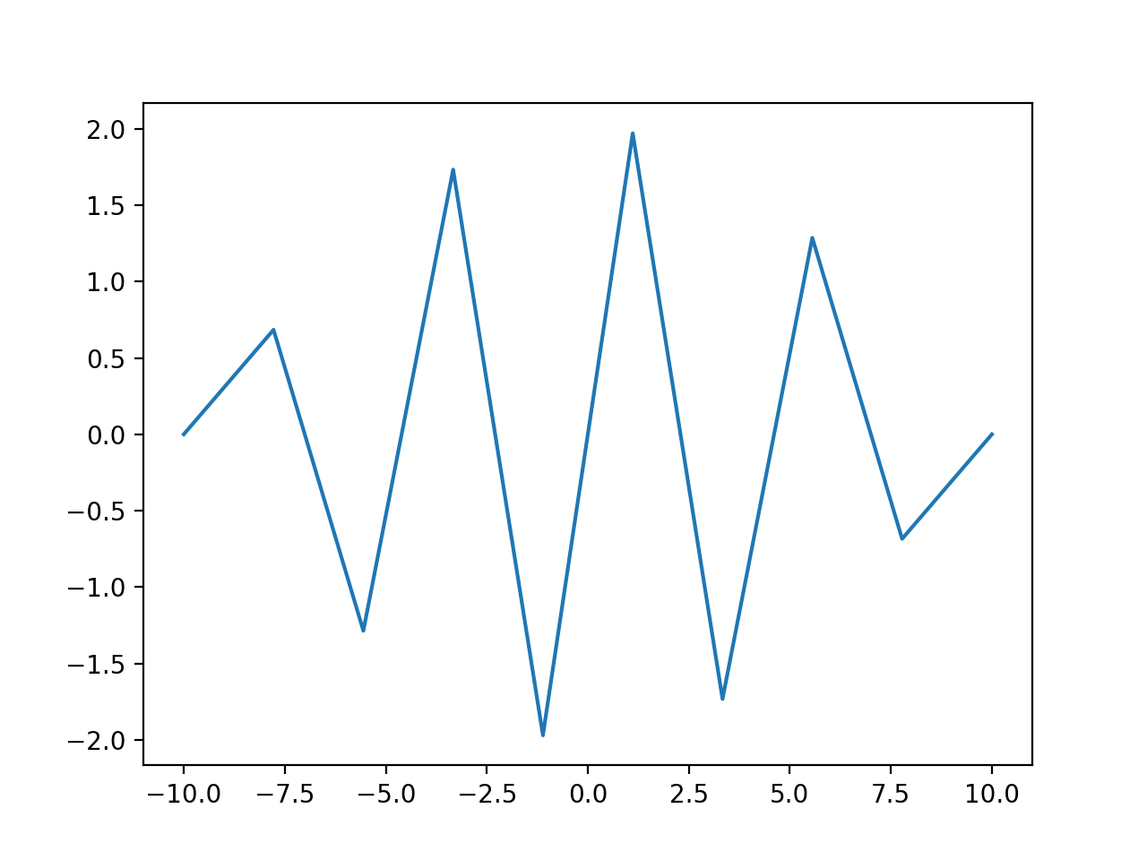
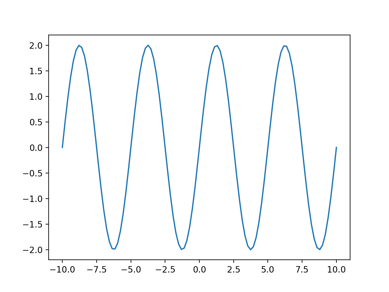
That doesn’t look like a sine wave, but you saw this issue earlier. The resolution of the linear space used for x_ isn’t sufficient. You can fix this by increasing the sampling:

x_ = np.linspace(-10, 10, 100)

wave = amplitude * np.sin((2*np.pi/wavelength) * (x_ - velocity*time))

plt.plot(x_, wave)
plt.show()

This plot of the wave now shows a smooth wave:

Now you’re ready to superimpose two waves. All you need to do is create two different waves and add them up. This is also a good time to refactor the code to tidy it up a bit:

import matplotlib.pyplot as plt
import numpy as np

# Parameters for discretizing the mathematical function
sampling = 100
x_range = -10, 10
n_waves = 2

# Parameters are tuples with a value for each wave (2 in this case)
amplitudes = 1.7, 0.8
wavelengths = 4, 7.5
velocities = 2, 1.5

time = 0  # You can set time to 0 for now

x_ = np.linspace(x_range[0], x_range[1], sampling)

# Create 2 (or more) waves using a list comprehension and superimpose
waves = [amplitudes[idx] * np.sin((2*np.pi/wavelengths[idx]) *
                                  (x_ - velocities[idx]*time))
         for idx in range(n_waves)]
superimposed_wave = sum(waves)

# Plot both waves separately to see what they look like
plt.subplot(2, 1, 1)
plt.plot(x_, waves[0])
plt.plot(x_, waves[1])

# Plot the superimposed wave
plt.subplot(2, 1, 2)
plt.plot(x_, superimposed_wave)

plt.show()

This code creates two different waves and adds them together, showing the superimposition of waves:

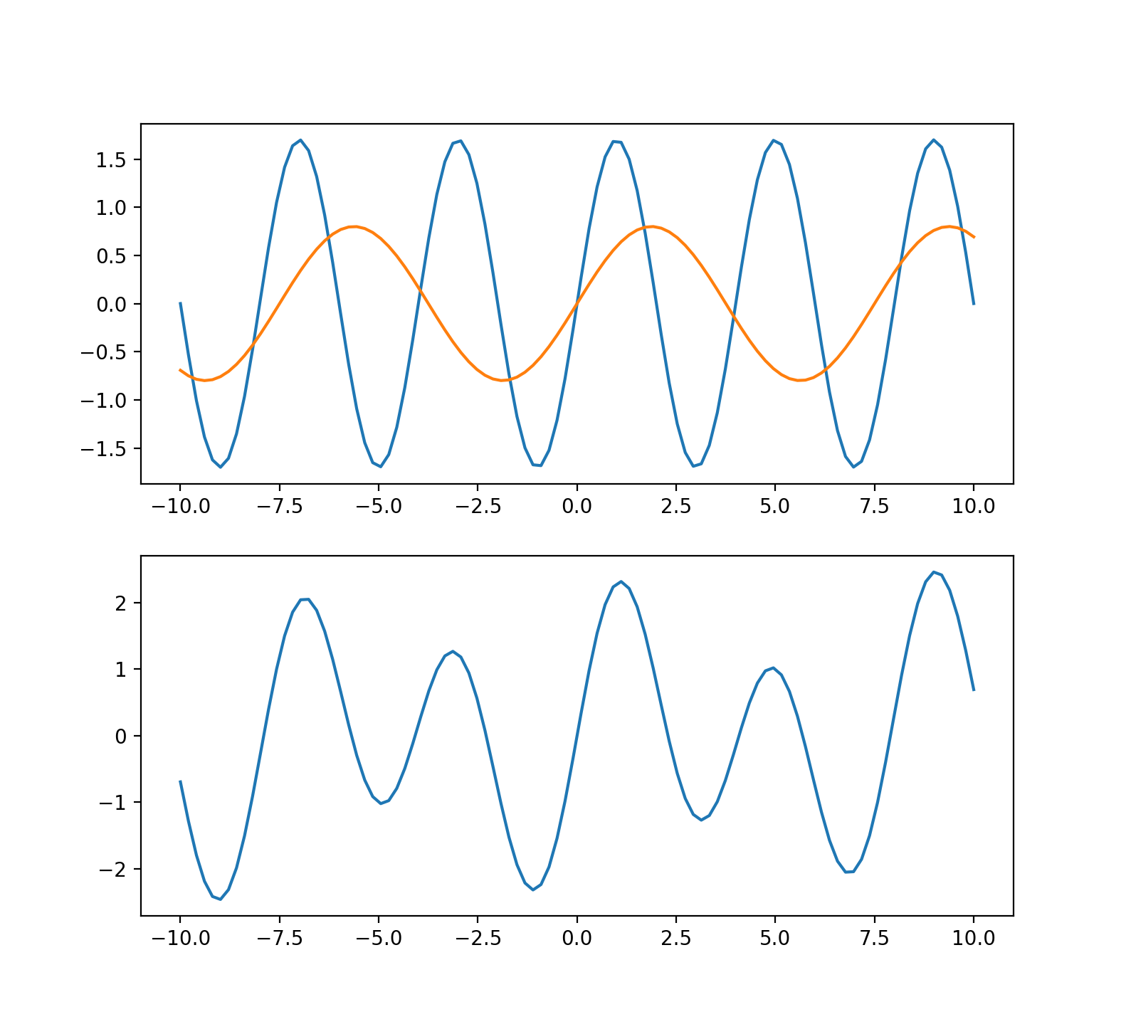
You can see both waves plotted separately in the top figure. The bottom figure shows the superimposition of the waves, when they’re added together. Your final task now is to set these waves in motion by plotting the superimposed waves for different values of time t:

for time in np.arange(0, 40, 0.2):
    # Create 2 (or more) waves using a list comprehension and superimpose
    waves = [amplitudes[idx] *
             np.sin((2*np.pi/wavelengths[idx]) *
                    (x_ - velocities[idx]*time))
             for idx in range(n_waves)]
    superimposed_wave = sum(waves)

    plt.clf()  # Clear last figure
    plt.plot(x_, superimposed_wave)
    plt.ylim(-3, 3)  # Fix the limits on the y-axis
    plt.pause(0.1)  # Insert short pause to create animation

This gives the following output:

You can try out the code above with waves of different parameters, and you can even add a third or fourth wave. You can now pick your own favorite functions to experiment with and try to represent them in Python.

Two-Dimensional Mathematical Functions

In the previous example, you resolved the problem of having a function with two variables by representing one as a spatial coordinate and one as a time coordinate. This made sense as the two coordinates were indeed one spatial and one temporal.

This method won’t always work, though. Here’s a function with two variables:

This is the simplified Gaussian function in two dimensions, with all parameters having unit value. To represent this, you’ll need to create two linear spaces, one for x and one for y. In this case, they can be identical, but that doesn’t always need to be the case:

import numpy as np

x_ = np.linspace(-5, 5, 100)
y_ = np.linspace(-5, 5, 100)

These vectors are each one-dimensional, but the required array must be two-dimensional since it needs to represent a function of two variables. NumPy has a useful function called np.meshgrid() that you can use in conjunction with np.linspace() to transform one-dimensional vectors into two-dimensional matrices. These matrices represent the coordinates in two dimensions:

>>> X, Y = np.meshgrid(x_, y_)
>>> x_.shape, y_.shape
((100,), (100,))
>>> X.shape, Y.shape
((100, 100), (100, 100))

You’ve transformed the vectors into two-dimensional arrays. You can now use these arrays to create the two-dimensional function:

gaussian = np.exp(-((X**2) / 2 + (Y**2) / 2))

You can show this matrix in two or three dimensions using matplotlib:

import matplotlib.pyplot as plt
from mpl_toolkits.mplot3d import Axes3D

fig = plt.figure()

ax = fig.add_subplot(121)
# Show matrix in two dimensions
ax.matshow(gaussian, cmap="jet")

ax = fig.add_subplot(122, projection="3d")
# Show three-dimensional surface
ax.plot_surface(X, Y, gaussian, cmap="jet")
plt.show()

The two-dimensional and three-dimensional representations are shown below:

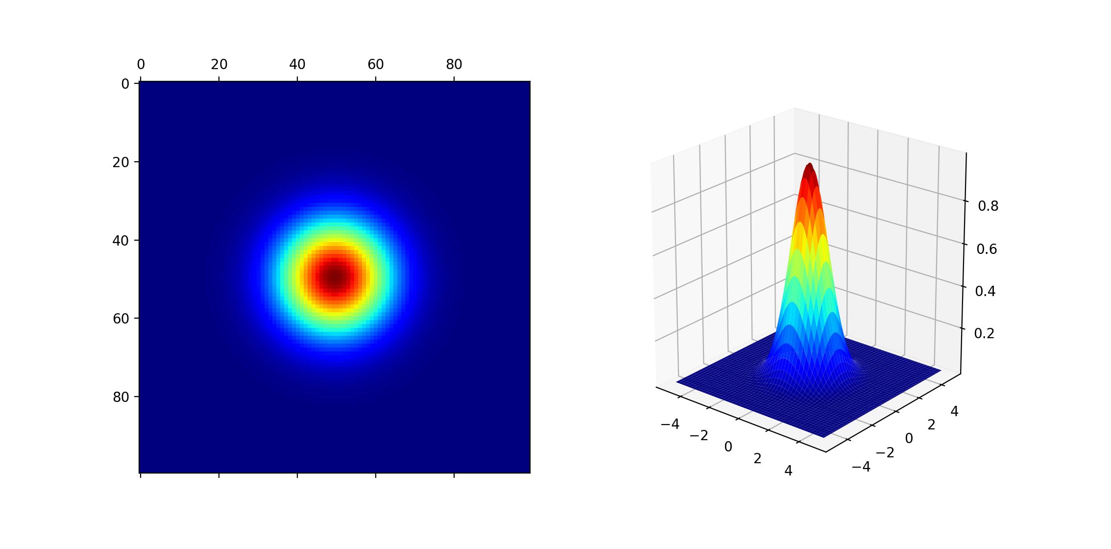
You can use this method for any function of two variables. If you wanted to create a binary disk-shaped mask, then you could represent this function using comparison operators:

 1import matplotlib.pyplot as plt
 2import numpy as np
 3
 4x_ = np.linspace(-10, 10, 1000)
 5y_ = np.linspace(-10, 10, 1000)
 6
 7X, Y = np.meshgrid(x_, y_)
 8
 9radius = 8
10disk_mask = (X ** 2) + (Y ** 2) < radius ** 2
11
12plt.matshow(disk_mask, cmap="gray", extent=[-10, 10, -10, 10])
13plt.show()

On line 10, you generate the array disk_mask using element-wise comparison. This gives the following plot:

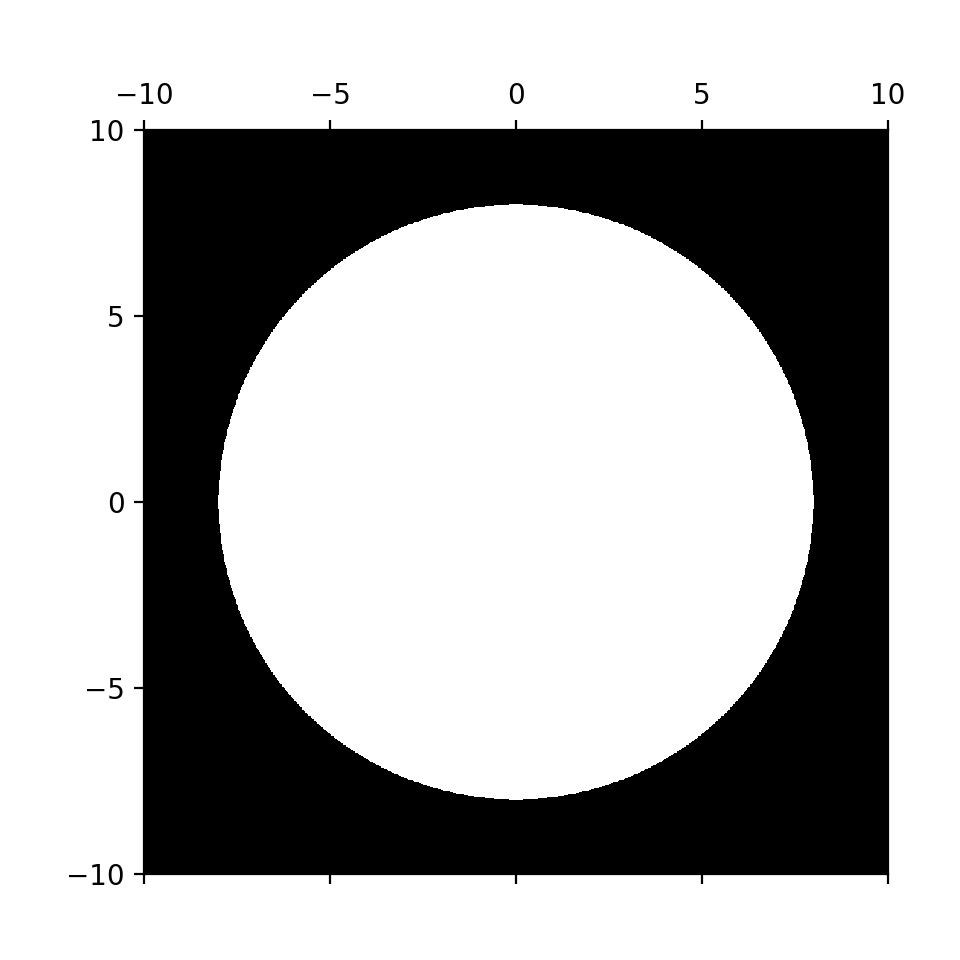
The array disk_mask has the value True (or 1) for all values of x_ and y_ that fall within the equation of the circle. Otherwise, it has the value False (or 0).

You’re now equipped with the tools to represent mathematical functions in one dimension and two dimensions computationally, using np.linspace() to create the linear spaces required to represent the function variables. You can extend the same concept to higher dimensions as well.

Logarithmic Spaces

The function np.logspace() creates a logarithmic space in which the numbers created are evenly spaced on a log scale.

Once you’ve mastered np.linspace(), you’ll be well equipped to use np.logspace() since the input parameters and returned output of the two functions are very similar. One parameter that’s missing from np.logspace() is retstep since there isn’t a single value to represent the step change between successive numbers.

np.logspace() has an additional input parameter, base, with a default value of 10. Another key difference is that start and stop represent the logarithmic start and end points. The first value in the array is basestart, and the final value is basestop:

>>> import numpy as np
>>> np.logspace(0, 4, 5)
array([1.e+00, 1.e+01, 1.e+02, 1.e+03, 1.e+04])

This creates a logarithmic space with 5 elements ranging from 100 to 104, or from 1 to 10000. The output array shows the numbers 1, 10, 100, 1000, and 10000 in scientific notation. Although base 10 is the default value, you can create logarithmic spaces with any base:

>>> np.logspace(1, 10, 20, base=np.e)
array([2.71828183e+00, 4.36528819e+00, 7.01021535e+00, 1.12577033e+01,
       1.80787433e+01, 2.90326498e+01, 4.66235260e+01, 7.48727102e+01,
       1.20238069e+02, 1.93090288e+02, 3.10083652e+02, 4.97963268e+02,
       7.99679103e+02, 1.28420450e+03, 2.06230372e+03, 3.31185309e+03,
       5.31850415e+03, 8.54098465e+03, 1.37159654e+04, 2.20264658e+04])

This example shows a logarithmic space in base e. In the next section, you’ll see how to create other nonlinear ranges that aren’t logarithmic.

Other Nonlinear Ranges

You can now create linear and logarithmic spaces. You may also need a range of numbers that follow other nonlinear intervals. You can achieve this by transforming a linear space.

Start by creating a linear space:

>>> import numpy as np
>>> x_ = np.linspace(1, 10, 10)
>>> x_
array([ 1.,  2.,  3.,  4.,  5.,  6.,  7.,  8.,  9., 10.])

You can now transform this to be a range of numbers that are linear over x²:

>>> x_ = x_ ** 2
>>> x_
array([  1.,   4.,   9.,  16.,  25.,  36.,  49.,  64.,  81., 100.])

This may seem familiar. It’s the same method you used to represent mathematical functions earlier in this tutorial. Indeed, it’s exactly the same. The reason you may sometimes want to think of this as creating a non-evenly spaced array will become clearer in the next section, when you look at a concrete example.

Example: Simulation of an Orbiting Planet

In this section, you’ll create a simulation of a planet orbiting around its sun. To simplify the simulation slightly, you can assume the planet’s orbit is circular rather than elliptical.

The equation that describes a circle is a function of x and y and depends on the radius R:

So if the x-positions of the planet are set, the corresponding y-positions will be given by rearranging the equation above:

The planet can therefore be placed at a set of coordinates (x, y), and as long as y is given by the equation above, the planet will remain in orbit. Its location will be on the circumference of a circle.

You’re now well versed with np.linspace(), so the first attempt can use the methods you already know:

import numpy as np

sampling = 50
R = 50

x_ = R * np.linspace(-1, 1, sampling)

The variable x spans the diameter of the circle along the horizontal, from left to right, which means from -R to +R. Now you can work out y:

y_ = np.sqrt(R ** 2 - x_ ** 2)

The array y_ is the discrete version of the continuous variable y, which describes a circle. You can plot these points using a scatter plot:

import matplotlib.pyplot as plt

plt.scatter(x_, y_)
plt.axis("square")
plt.show()

To make sure the two-dimensional plot shows the correct pattern, you set the axes to "square", which ensures that each pixel has a square aspect ratio:

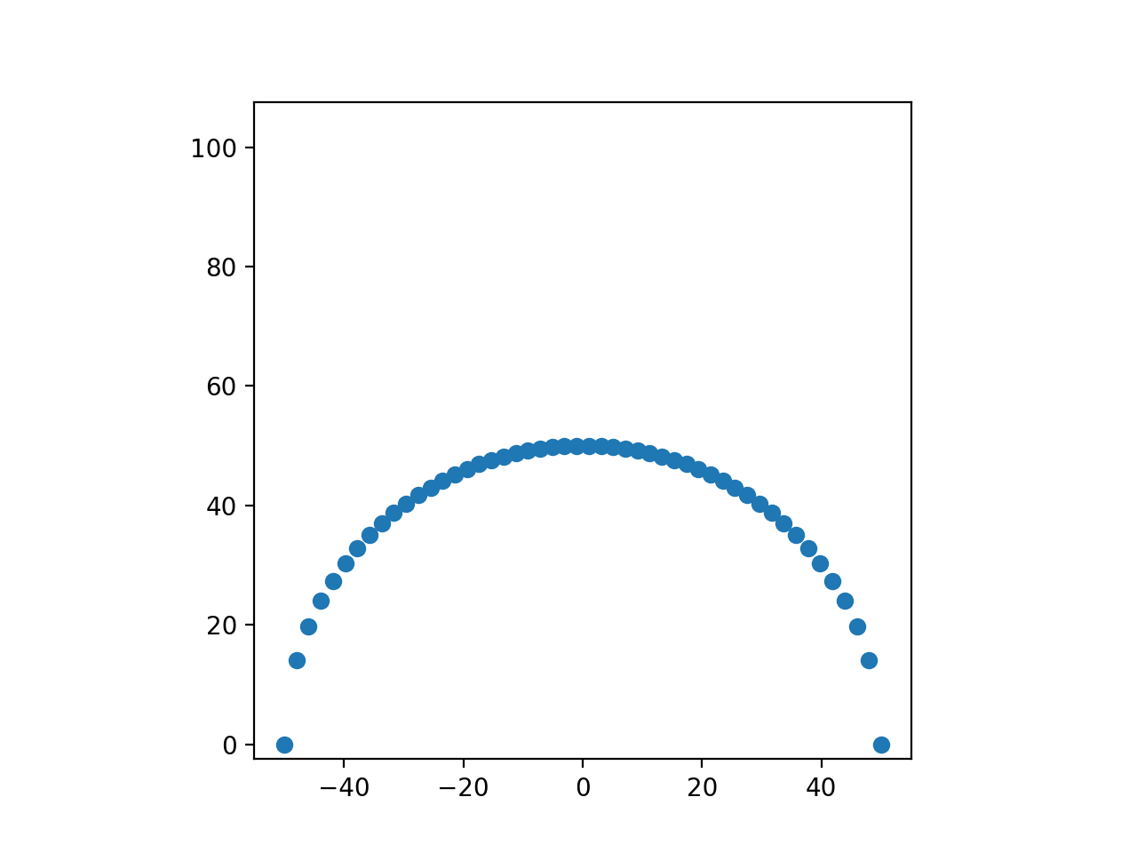
All points fit nicely on the circumference of a circle, which should be the case for a planet in a circular orbit.

But planets don’t only go around a semicircular orbit. The problem is that the values of x for the other half of the circle are the same. The top semicircle and the bottom one share the same x values but not the same y values.

You can resolve this issue by looking back at the above equation that gives y in terms of x. This equation has both a positive solution and a negative one. As x swings back from +R on the right to -R on the left, you can take the negative solution for y:

# x_return and y_return are the x_ and y_ values as the
# planet moves from right to left
x_return = x_[len(x_)-2:0:-1]
y_return = -np.sqrt(R ** 2 - x_return ** 2)

x_ = np.concatenate((x_, x_return))
y_ = np.concatenate((y_, y_return))

The array x_return is the reverse of x_ but without the endpoints. Otherwise, the endpoints will be repeated when you concatenate x_ and x_return. The array y_return is the negative solution for y_. Therefore, you can overwrite x_ to become the concatenation of x_ and x_return:

>>> x_
array([-50.        , -47.95918367, -45.91836735, -43.87755102,
       -41.83673469, -39.79591837, -37.75510204, -35.71428571,
       -33.67346939, -31.63265306, -29.59183673, -27.55102041,
       -25.51020408, -23.46938776, -21.42857143, -19.3877551 ,
       -17.34693878, -15.30612245, -13.26530612, -11.2244898 ,
        -9.18367347,  -7.14285714,  -5.10204082,  -3.06122449,
        -1.02040816,   1.02040816,   3.06122449,   5.10204082,
         7.14285714,   9.18367347,  11.2244898 ,  13.26530612,
        15.30612245,  17.34693878,  19.3877551 ,  21.42857143,
        23.46938776,  25.51020408,  27.55102041,  29.59183673,
        31.63265306,  33.67346939,  35.71428571,  37.75510204,
        39.79591837,  41.83673469,  43.87755102,  45.91836735,
        47.95918367,  50.        ,  47.95918367,  45.91836735,
        43.87755102,  41.83673469,  39.79591837,  37.75510204,
        35.71428571,  33.67346939,  31.63265306,  29.59183673,
        27.55102041,  25.51020408,  23.46938776,  21.42857143,
        19.3877551 ,  17.34693878,  15.30612245,  13.26530612,
        11.2244898 ,   9.18367347,   7.14285714,   5.10204082,
         3.06122449,   1.02040816,  -1.02040816,  -3.06122449,
        -5.10204082,  -7.14285714,  -9.18367347, -11.2244898 ,
       -13.26530612, -15.30612245, -17.34693878, -19.3877551 ,
       -21.42857143, -23.46938776, -25.51020408, -27.55102041,
       -29.59183673, -31.63265306, -33.67346939, -35.71428571,
       -37.75510204, -39.79591837, -41.83673469, -43.87755102,
       -45.91836735, -47.95918367])

The values within x_ go from -50 through 0 to 50 and then back through 0 to -50. You can also print y_ to confirm that it corresponds to the positive values of y for the first half and the negative values of y for the second half. A scatter plot of x_ and y_ will confirm that the planet is now in an orbit that’s a full circle:

plt.scatter(x_, y_)
plt.axis("square")
plt.show()

This gives the following plot:

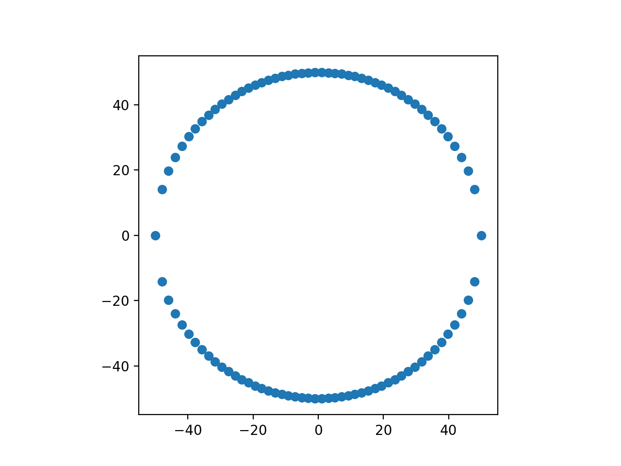
You may already be able to spot the problem in this scatter plot, but you’ll come back to it a bit later. For now, you can use the x_ and y_ vectors above to create a simulation of the moving planet.

You’ll need to import matplotlib.animation for this:

import matplotlib.animation

# Create a figure and axis handle, set axis to
# an equal aspect (square), and turn the axes off
fig, ax = plt.subplots()
ax.set_aspect("equal")
ax.set_axis_off()

# Images are generated and stored in a list to animate later
images = []
for x_coord, y_coord in zip(x_, y_):
    # Scatter plot each point using a dot of size 250 and color red
    img = ax.scatter(x_coord, y_coord, s=250, c="r")
    # Let's also put a large yellow sun in the middle
    img2 = ax.scatter(0, 0, s=1000, c="y")
    images.append([img, img2])

# The animation can now be created using ArtistAnimation
animation = matplotlib.animation.ArtistAnimation(fig,
                                                 images,
                                                 interval=2.5,
                                                 blit=True
                                                 )
plt.show()

This gives the following output:

Unfortunately, planets don’t orbit in this manner. You can see how the planet speeds up as it crosses the x-axis at the left and right of the orbit and slows down as it crosses the y-axis at the top and bottom.

Take another look at the scatter plots showing all the planet positions around the orbit to see why this happens. The points are closer together at the top and bottom of the orbit but spaced out on the left and right. You need points that are evenly spaced over the circumference of the orbit, but what you have are points based on an evenly spaced x_ vector.

To fix this, you need to create an array of x_ values that isn’t linear but that produces points that are linear along the circumference of the orbit. As a point moves smoothly around a circular orbit, its projection on the x-axis moves (co-)sinusoidally, so you can fix this by changing x_ so that it’s linear over cos(x_):

x_ = R * np.cos(np.linspace(-np.pi, 0, sampling))
x_return = x_[len(x_)-2: 0: -1]

y_ = np.sqrt(R ** 2 - x_ ** 2)
y_return = -np.sqrt(R ** 2 - x_return ** 2)

x_ = np.concatenate((x_, x_return))
y_ = np.concatenate((y_, y_return))

plt.scatter(x_, y_)
plt.axis("square")
plt.show()

The first line transforms a linear space into a nonlinear one. The intervals between each value of x_ aren’t equal but vary according to the cosine function. This gives the following plot:

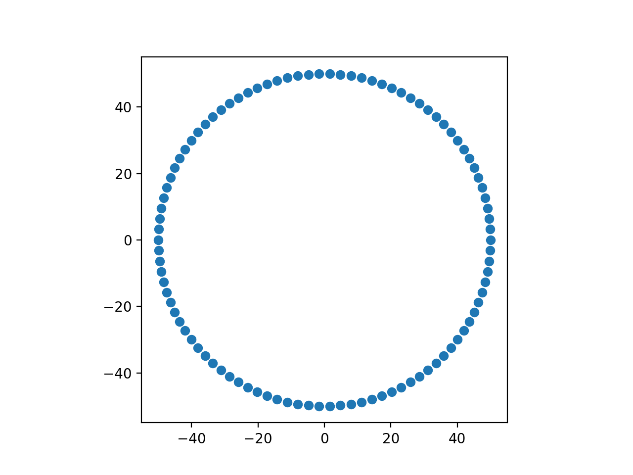
The points are now evenly spaced across the circumference of the circular orbit. Your final step is to re-create the animation using the same code as earlier. This is also a good time to increase the resolution by increasing the value of the sampling variable you defined at the start:

sampling = 250

# ...

fig, ax = plt.subplots()
ax.set_aspect("equal")
ax.set_axis_off()

images = []
for x_coord, y_coord in zip(x_, y_):
    img = ax.scatter(x_coord, y_coord, s=250, c="r")
    img2 = ax.scatter(0, 0, s=1000, c="y")
    images.append([img, img2])

animation = matplotlib.animation.ArtistAnimation(fig,
                                                 images,
                                                 interval=2.5,
                                                 blit=True
                                                 )
plt.show()

This gives the following output:

To see the full version of the code that generates this animation, you can expand the section below.

 1import matplotlib.animation
 2import matplotlib.pyplot as plt
 3import numpy as np
 4
 5sampling = 250
 6R = 50
 7
 8# Create vector x_ that is linear on cos(x_)
 9# First create x_ from left to right (-R to +R)
10x_ = R * np.cos(np.linspace(-np.pi, 0, sampling))
11# And then x_ returns from right to left (+R to R)
12x_return = x_[len(x_)-2: 0: -1]
13
14# Calculate y_ using the positive solution when x_ is increasing
15y_ = np.sqrt(R ** 2 - x_ ** 2)
16# And the negative solution when x_ is decreasing
17y_return = -np.sqrt(R ** 2 - x_return ** 2)
18
19x_ = np.concatenate((x_, x_return))
20y_ = np.concatenate((y_, y_return))
21
22# Create animation
23fig, ax = plt.subplots()
24ax.set_aspect("equal")
25ax.set_axis_off()
26
27images = []
28for x_coord, y_coord in zip(x_, y_):
29    img = ax.scatter(x_coord, y_coord, s=250, c="r")
30    img2 = ax.scatter(0, 0, s=1000, c="y")
31    images.append([img, img2])
32
33animation = matplotlib.animation.ArtistAnimation(fig,
34                                                 images,
35                                                 interval=2.5,
36                                                 blit=True
37                                                 )
38plt.show()
39
40# Export to .gif
41writer = matplotlib.animation.PillowWriter(fps=30)
42animation.save("orbiting_planet_simulation.gif", writer=writer)

You’ve just created an animation of a planet orbiting a star. You had to make the movement of the planet linear over the circumference of a circle by making the positions of the planet evenly spaced over the circumference of the circle. You can now create any non-evenly spaced range of numbers as long as you can express it mathematically.